Decorrelation penalty

ctrl_lambda penalises the dependence between a model's predictions and one or more control variables. The inputs are:

• X: the input features;

• Y: the target;

• C: a control variable whose dependence with the predictions should be reduced. C may or may not be one of the features.

Dependence is measured by distance covariance, which also captures nonlinear dependence. The design notes describe how the penalty is defined and computed.

Data

Y depends on C only through its square. C is not a feature, but the first feature is a noisy measurement of it, so a model can learn that dependence. Y0 is the part of Y that does not depend on C. Rows come in groups of 200, identified by group.

using EvoTrees, Random, Statistics, Printf

function simulate(rng; ngroups=200, group_size=200)
    n = ngroups * group_size
    group = repeat(1:ngroups, inner=group_size)
    c = randn(rng, n)
    x = hcat(c .+ 0.2 .* randn(rng, n), randn(rng, n, 3))
    y0 = x[:, 2] .+ 0.5 .* x[:, 3] .+ 0.5 .* x[:, 4]
    y = y0 .+ 0.8 .* (c .^ 2 .- 1) .+ 0.5 .* randn(rng, n)
    return (; x, y, y0, c, group)
end

rng = Xoshiro(1)
train, valid, test = simulate(rng), simulate(rng), simulate(rng)

Fitting with the penalty

Pass the control as ctrl_train, one value per row, or from a table as the column name ctrl_name. That column is not used as a feature unless listed in feature_names.

config(λ) = EvoTreeRegressor(loss=:mse, nrounds=200, eta=0.05, max_depth=5, ctrl_lambda=λ)

m0 = EvoTrees.fit(config(0.0); x_train=train.x, y_train=train.y, verbosity=0)
m1 = EvoTrees.fit(config(30.0); x_train=train.x, y_train=train.y, ctrl_train=train.c, verbosity=0)

On the test set, compare the Pearson correlation and the squared distance correlation (EvoTrees.dcor2) of the predictions with C, and their correlation with Y and Y0:

for (name, m) in (("no penalty", m0), ("ctrl_lambda = 30", m1))
    p = m(test.x)
    @printf("%-16s  cor(p, C) %.3f  dcor2(p, C) %.3f  cor(p, Y) %.3f  cor(p, Y0) %.3f\n", name,
        cor(p, test.c), EvoTrees.dcor2(p, test.c), cor(p, test.y), cor(p, test.y0))
end

no penalty        cor(p, C) 0.012  dcor2(p, C) 0.085  cor(p, Y) 0.926  cor(p, Y0) 0.754
ctrl_lambda = 30  cor(p, C) 0.007  dcor2(p, C) 0.016  cor(p, Y) 0.860  cor(p, Y0) 0.902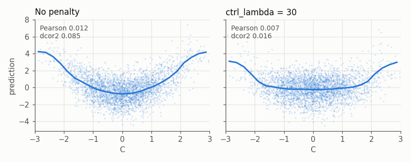

Without the penalty the predictions follow the square of C (left), yet their Pearson correlation with C is near zero. The distance correlation captures this dependence, and the penalty removes most of it. The predictions then track Y0 more closely and Y less, since part of Y comes from C.

Within groups

To remove the dependence within each group only, set ctrl_within_group = true and pass the group ids. The control is then standardised and the penalty computed within each group.

config_g = EvoTreeRegressor(loss=:mse, nrounds=200, eta=0.05, max_depth=5,
    ctrl_lambda=30.0, ctrl_within_group=true)
m2 = EvoTrees.fit(config_g; x_train=train.x, y_train=train.y, ctrl_train=train.c,
    group_train=train.group, verbosity=0)

rows = [findall(==(g), test.group) for g in unique(test.group)]
for (name, m) in (("no penalty", m0), ("within groups", m2))
    p = m(test.x)
    @printf("%-14s  mean dcor2(p, C) within groups %.3f\n", name,
        mean(EvoTrees.dcor2(p[r], test.c[r]) for r in rows))
end

no penalty      mean dcor2(p, C) within groups 0.084
within groups   mean dcor2(p, C) within groups 0.016

The groups here have no structure of their own, so the result is close to the pooled fit. The two forms differ when C or Y has a group-level component, which only the pooled penalty acts on.

Choosing ctrl_lambda

Fit a few weights and compare them on validation data. The error rises as the dependence falls:

for λ in (0.0, 3.0, 10.0, 30.0, 100.0, 300.0)
    m = EvoTrees.fit(config(λ); x_train=train.x, y_train=train.y, ctrl_train=train.c, verbosity=0)
    p = m(valid.x)
    @printf("ctrl_lambda %5g  mse %.3f  cor(p, C) %+.3f  dcor2(p, C) %.4f\n", λ,
        mean((p .- valid.y) .^ 2), cor(p, valid.c), EvoTrees.dcor2(p, valid.c))
end

ctrl_lambda     0  mse 0.430  cor(p, C) -0.000  dcor2(p, C) 0.0833
ctrl_lambda     3  mse 0.450  cor(p, C) -0.002  dcor2(p, C) 0.0640
ctrl_lambda    10  mse 0.556  cor(p, C) -0.003  dcor2(p, C) 0.0382
ctrl_lambda    30  mse 0.805  cor(p, C) -0.004  dcor2(p, C) 0.0147
ctrl_lambda   100  mse 1.151  cor(p, C) -0.003  dcor2(p, C) 0.0035
ctrl_lambda   300  mse 4.265  cor(p, C) +0.159  dcor2(p, C) 0.0229

Past some ctrl_lambda * eta, between 5 and 15 here, the fit oscillates instead of settling, as at 300, so a larger weight needs a smaller eta. The weight also scales with the target: a target 10 times larger needs about 10 times the weight.

Several controls

ctrl_train also takes a matrix with one column per control, and ctrl_name a vector of names. Each control adds its own term, multiplied by its entry in ctrl_weights. Here the fourth feature is added as a second control with half the weight:

m3 = EvoTrees.fit(config(30.0); x_train=train.x, y_train=train.y,
    ctrl_train=hcat(train.c, train.x[:, 4]), ctrl_weights=[1.0, 0.5], verbosity=0)

for (name, m) in (("no penalty", m0), ("C", m1), ("C and X4", m3))
    p = m(test.x)
    @printf("%-10s  dcor2(p, C) %.3f  dcor2(p, X4) %.3f\n", name,
        EvoTrees.dcor2(p, test.c), EvoTrees.dcor2(p, test.x[:, 4]))
end

no penalty  dcor2(p, C) 0.085  dcor2(p, X4) 0.088
C           dcor2(p, C) 0.016  dcor2(p, X4) 0.124
C and X4    dcor2(p, C) 0.017  dcor2(p, X4) 0.006

Penalising C alone makes the model lean more on the fourth feature, and the second control limits that. Since the terms are summed, a dependence that shows only in a combination of controls is not penalised.

Early stopping

With evaluation data, the loss's own metric includes the penalty, so early stopping follows the penalised objective. The evaluation data needs the same controls (ctrl_eval, or the ctrl_name columns in deval), and its groups under ctrl_within_group.

config_es = EvoTreeRegressor(loss=:mse, nrounds=2000, eta=0.05, max_depth=5,
    ctrl_lambda=30.0, early_stopping_rounds=50)
m4 = EvoTrees.fit(config_es; x_train=train.x, y_train=train.y, ctrl_train=train.c,
    x_eval=valid.x, y_eval=valid.y, ctrl_eval=valid.c, verbosity=0)

logger = m4.info[:logger]
i = logger[:best_iter] + 1
@printf("best round %d: mse %.4f, dependence %.5f, penalised %.4f\n", logger[:best_iter],
    logger[:base_metrics][i], logger[:ctrl_dependence][i][1], logger[:metrics][i])

best round 281: mse 0.8030, dependence 0.00793, penalised 1.0408

The penalised value is the mse plus ctrl_lambda times the dependence, dcov2 of the predictions and the standardised control. The logger keeps both parts for every round under :base_metrics and :ctrl_dependence. Other metrics, such as :mae, are reported unchanged.

Other losses and devices

The penalty is available on EvoTreeRegressor for :mse, :logloss, :poisson, :gamma, :tweedie and, within groups only, :pearson, and on EvoTreeMLE for :gaussian_mle, where it acts on the location. Under losses other than :mse its gradient is weighted by the loss's curvature, so a given weight has about the same effect. Under :pearson the default metric, :pearson, does not include the penalty, while metric = :pearson_mse, the loss's objective, does. On GPU the penalty is computed on the host. The MLJ interface cannot pass controls, so the penalty is only available through EvoTrees.fit.