NeuroTree - A differentiable tree operator for tabular data

Overview

This work introduces NeuroTree a differentiable binary tree operator adapted for the treatment of tabular data.

• Address the shortcoming of traditional trees greediness: all node and leaves are learned simultaneously. It provides the ability to learn an optimal configuration across all of the tree levels.

The notion extent also to the collection of trees that are simultaneously learned.

• Extend the notion of forest/bagging and boosting.

  • Although the predictions from the all of of the trees forming a NeuroTree operator are averaged, each of the tree prediction tuned simultaneously. This is different from boosting (ex XGBoost) where each tree is learned sequentially and over the residual from previous trees. Also, unlike random forest and bagging, trees aren't learned in isolation but tuned collaboratively, resulting in predictions that account for all of the other trees predictions.

• General operator compatible for composition.

  • Allows integration within Flux's Chain like other standard operators from NNLib. Composition is also illustrated through the built-in StackTree layer, a residual composition of multiple NeuroTree building blocks.

• Compatible with general purpose machine learning framework.

  • MLJ integration

Architecture

To introduce the implementation of a NeuroTree, we first get back to the architecture of a basic decision tree.

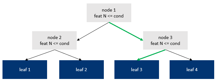
The above is a binary decision tree of depth 2.

Highlighted in green is the decision path taken for a given sample. It goes into depth number of binary decisions, resulting in the path node1 → node3 → leaf3.

One way to view the role of the decision nodes is to provide an index of the leaf prediction to fetch (index 3 in the figure). Such indexing view is applicable given that node routing relies a hard conditions: it's either true or false.

An alternative perspective that we will adopt here is that tree nodes collectively provide weights associated to each leaf. A tree prediction is the weighted sum of the leaf's value and those leaf weights. In regular decision trees, since all conditions are binary, leaf weights take the form of a mask. In the above example, the mask is [0, 0, 1, 0].

By relaxing these these hard condition into soft ones, the mask takes the form of a probability vector associated to each leaf, where ∑(leaf_weights) = 1 and where each each leaf_weight element is [0, 1].

The following illustrate how a basic decision tree is represented as a single differentiable tree within NeuroTree:

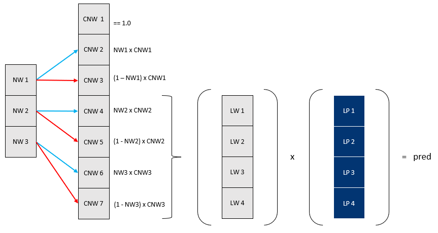
Node weights

To derive how a NeuroTree performs those soft decision, we first break down the structure of how the traditional hard decisions are taken. A nodes's split actually relies on 2 binary conditions:

1. Selection of the feature on which to perform the condition

The selection of a feature out of the selected ones In NeuroTree, these hard decisions are translated into soft, differentiable ones: 1.

2. Selection of the condition's threshold value

A NeuroTree operator acts as collection of complete binary trees, ie. trees without any pruned node. In order to be differentiable, hence trainable using gradient based methods such as Adam, each tree path implements a soft decision rather than a hard one like in traditional decision tree.

Leaf weights

Computing the leaf weights consists of accumulating the weights through each tree branch. It's the technically more challenging part as such computation cannot be represented as a form of matrix multiplication, unlike other common operators like Dense, Conv or MultiHeadAttention / Transformer. Performing probability accumulation though a tree index naturally leads to in-place element wise operations, which are notoriously not friendly for auto-differentiation engines. Since NeuroTree was intended to integrate with the Flux.jl ecosystem, Zygote.jl acts as the underlying AD, the approach used was to to manually implement backward / adjoint of the terminal leaf function and instruct the AD to use that custom rule rather than attempt to differentiate a non-AD compliant function.

Below are the algo and actual implementation of the forward and backward function that compute the leaf weights. For brevity, the loops over each observation of the batch and each tree are omitted. Parallelism, both on CPU and GPU, is obtained through parallelization over the tree and batch dimensions.

Forward

function leaf_weights!(nw)
    cw = ones(eltype(nw), 2 * size(nw, 1) + 1)

    for i = 2:2:size(cw, 1)
        cw[i] = cw[i>>1] * nw[i>>1]
        cw[i+1, tree, batch] = cw[i>>1] * (1 - nw[i>>1])
    end
    
    lw = cw[size(nw, 1)+1:size(cw, 1)]
    return (cw, lw)
end

Backward

function Δ_leaf_weights!(Δnw, ȳ, cw, nw, max_depth, node_offset)
    
    for i in axes(nw, 1)        
        depth = floor(Int, log2(i)) # current depth level - starting at 0
        step = 2^(max_depth - depth) # iteration length
        leaf_offset = step * (i - 2^depth) # offset on the leaf row

        for j = (1+leaf_offset):(step÷2+leaf_offset)
            k = j + node_offset # move from leaf position to full tree position 
            Δnw[i] += ȳ[j] * cw[k] / nw[i]
        end
    
        for j = (1+leaf_offset+step÷2):(step+leaf_offset)
            k = j + node_offset
            Δnw[i] -= ȳ[j] * cw[k] / (1 - nw[i])
        end
    end

    return nothing
end

Tree prediction

Composability

• StackTree

• General operator: Chain neurotree with MLP

Benchmarks

For each dataset and algo, the following methodology is followed:

• Data is split in three parts: train, eval and test

• A random grid of 16 hyper-parameters is generated

• For each parameter configuration, a model is trained on train data until the evaluation metric tracked against the eval stops improving (early stopping)

• The trained model is evaluated against the test data

• The metric presented in below are the ones obtained on the test for the model that generated the best eval metric.

Source code available at MLBenchmarks.jl.

For performance assessment, benchmarks is run on the following selection of common Tabular datasets:

• Year: min squared error regression

• MSRank: ranking problem with min squared error regression

• YahooRank: ranking problem with min squared error regression

• Higgs: 2-level classification with logistic regression

• Boston Housing: min squared error regression

• Titanic: 2-level classification with logistic regression

Comparison is performed against the following algos (implementation in link) considered as state of the art on classification tasks:

• EvoTrees

• XGBoost

• LightGBM

• CatBoost

• NODE

Boston

model_type	train_time	mse	gini
neurotrees	12.8	18.9	0.947
evotrees	0.206	19.7	0.927
xgboost	0.0648	19.4	0.935
lightgbm	0.865	25.4	0.926
catboost	0.0511	13.9	0.946

Titanic

model_type	train_time	logloss	accuracy
neurotrees	7.58	0.407	0.828
evotrees	0.673	0.382	0.828
xgboost	0.0379	0.375	0.821
lightgbm	0.615	0.390	0.836
catboost	0.0326	0.388	0.836

Year

model_type	train_time	mse	gini
neurotrees	280.0	76.4	0.652
evotrees	18.6	80.1	0.627
xgboost	17.2	80.2	0.626
lightgbm	8.11	80.3	0.624
catboost	80.0	79.2	0.635

MSRank

model_type	train_time	mse	ndcg
neurotrees	39.1	0.578	0.462
evotrees	37.0	0.554	0.504
xgboost	12.5	0.554	0.503
lightgbm	37.5	0.553	0.503
catboost	15.1	0.558	0.497

Yahoo

model_type	train_time	mse	ndcg
neurotrees	417.0	0.584	0.781
evotrees	687.0	0.545	0.797
xgboost	120.0	0.547	0.798
lightgbm	244.0	0.540	0.796
catboost	161.0	0.561	0.794

Higgs

model_type	train_time	logloss	accuracy
neurotrees	12300.0	0.452	0.781
evotrees	2620.0	0.464	0.776
xgboost	1390.0	0.462	0.776
lightgbm	1330.0	0.461	0.779
catboost	7180.0	0.464	0.775

References

• Neural Oblivious Decision Ensembles for Deep Learning on Tabular Data.

  • https://github.com/Qwicen/node

  • https://github.com/manujosephv/pytorch_tabular

• Attention augmented differentiable forest for tabular data

• NCART: Neural Classification and Regression Tree for Tabular Data

• Squeeze-and-Excitation Networks

• Deep Neural Decision Trees

• XGBoost: A Scalable Tree Boosting System

• CatBoost: gradient boosting with categorical features support

• LightGBM: A Highly Efficient Gradient Boosting Decision Tree

• Deep Neural Decision Trees

• Neural Decision Trees